Internal development / TSC Simulation
Pipe Friction and Pressure-Drop Modelling.
Owned development and simulator testing of a C-based SimEdit pipe-friction item, revisiting modelling assumptions to represent pressure loss and gas flow more accurately.
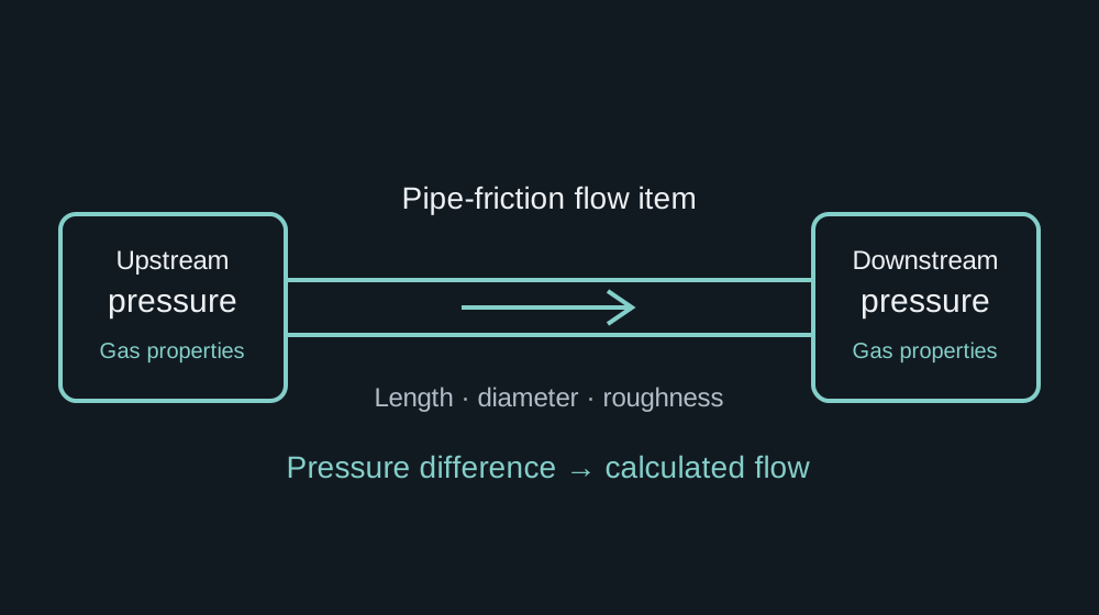
Method illustration by Luke Johnson
Turning a pressure difference into a flow
This internal development connected my engineering-study work with the underlying simulation platform. The task was to create a gas pipe-friction flow item: given pressures on either side, pipe dimensions, roughness and gas properties, calculate the flow between connected parts of the model.
The work drew on the AMEC gas-system studies and continued beyond the earlier Hole House Phase 3 study. Work began with friction-factor investigations in September 2011, followed by the dedicated item and further comparisons during May–July 2012.
Why the item was needed
A follow-up engineering investigation prompted a review of pressure-loss assumptions in an existing gas-system model. The original scope had adopted a simplified treatment of connecting pipework. Revisiting that assumption showed the need to represent distributed flow resistance explicitly, rather than treating the wider network as an equivalent pressure boundary.
The task therefore went beyond choosing a friction-factor equation: it required reconsidering where the model boundaries sat and which physical effects needed to be included.
As owner and developer of the item, I took it from method investigation and spreadsheet comparisons through to C implementation, with support from senior engineers and developer colleagues. Testing within the simulator used operating data to check the revised model’s behaviour with those losses represented.
The engineering problem
In a process simulation, a pressure or volume node represents gas inventory and its changing state. A flow node calculates the transfer between those inventories. This item provided the pressure-to-flow relationship using pipe-friction methods, rather than representing the connection through a large valve characteristic.
Its inputs included upstream and downstream pressures, gas temperature, composition and properties, plus pipe length, internal diameter and absolute roughness. The implementation selected the supplying side from the pressure direction and provided forward and reverse flow outputs.
Darcy–Weisbach as the starting point
For a straight, circular pipe with a representative constant density, the frictional pressure loss is:
Here, Δp is frictional pressure loss in pascals, fD is the dimensionless Darcy friction factor, L and D are pipe length and internal diameter in metres, ρ is density in kg/m³, and v is mean velocity in m/s. The friction term alone does not include elevation, fittings or acceleration effects.
Rearranging gives a velocity magnitude for a known pressure difference:
Flow direction follows the pressure difference. Cross-sectional area then connects velocity to volumetric and mass flow:
The friction factor is coupled to the velocity through Reynolds number, so selecting a friction calculation and solving the pressure-to-flow relationship need to be considered together.
Reynolds number, roughness and flow regime
Dynamic viscosity μ is expressed in Pa·s. The other important input is relative roughness, ε/D, where ε is the absolute internal roughness in metres.
For fully developed laminar flow in a circular pipe:
I used a laminar boundary of Re = 2,100 and a turbulent boundary of Re = 4,000, with interpolation between the endpoint friction factors. This gave the item a practical numerical treatment of transition, where the actual flow behaviour is less predictable.
The friction-factor convention matters throughout: the Darcy factor is four times the Fanning factor. Mixing the two changes the predicted pressure loss by a factor of four.
Turbulent friction and the choice of approximation
The Colebrook–White relation connects turbulent friction to Reynolds number and roughness:
The logarithm is base 10. Because fD appears on both sides, the relation normally requires an iterative solution. Explicit approximations offer a useful trade-off when a simulation evaluates many connections repeatedly.
| Method | Engineering role and limitation |
|---|---|
| Colebrook–White | A turbulent-flow reference that includes roughness. Solving it more closely reduces numerical equation-solving error, not uncertainty in the real pipe. |
| Existing internal approximation | A roughness-aware calculation I adapted from TSC’s platform alongside the Churchill option. |
| Churchill | A correlation covering laminar, transitional and turbulent regimes. The item used its own regime selection and interpolation around the selected friction method. |
| Blasius | A simple smooth-pipe turbulent approximation. It has no roughness term and becomes unsuitable when roughness materially affects the resistance. |
| Haaland and Swamee–Jain | Useful alternatives when choosing an explicit Colebrook approximation. I have included their equations for comparison; I did not implement these methods in this item. |
For smooth-pipe turbulent flow, a common Blasius form is:
The familiar quarter-power form is typically used over roughly Re = 4,000–100,000 for hydraulically smooth pipes. It is useful when that assumption and range fit the problem. It should not be extrapolated across rough-pipe or high-Reynolds-number conditions simply because the calculation is inexpensive.
Explicit approximation equations
Haaland provides a compact turbulent-flow approximation:
The Swamee–Jain form is another explicit turbulent-flow option:
Churchill’s correlation, written in the Darcy convention, uses the auxiliary quantities A and B below. These symbols belong only to this correlation.
Future considerations
For this work, we accepted the constant-density assumption and ruled compressibility effects on pressure drop out of scope. I used that basis for the item’s application and testing in the simulator.
If I revisited the item for connections with larger density changes, I would review gas expansion, temperature and compressibility before choosing the flow formulation. One possible starting point is the horizontal isothermal relationship below. It assumes constant temperature, compressibility factor and friction factor along the pipe, and neglects acceleration:
Here p₁ and p₂ are absolute pressures in pascals, Z is compressibility factor, Rs is the gas-specific constant in J/(kg·K), and T is absolute temperature in kelvin. I have included this equation to illustrate a possible extension; I did not implement compressibility effects for this work.
The worksheet comparisons explored alternative velocity formulations, but the simulator work retained the accepted constant-density basis. Extending the item would need a fresh check of the assumptions, friction convention and validation cases.
I also considered Panhandle A and B before simplifying the method set. These empirical gas-transmission correlations would be further options to assess for a suitable pipeline application, with careful attention to their assumptions, units and reference gas conditions.
Implementation in SimEdit
The C item fitted into TSC’s existing item-library structure, with an initialisation routine and a runtime calculation called by the simulation. Configuration fields exposed the pipe geometry, roughness and method choices; diagnostic values included Reynolds number, flow regime, friction factor, velocity estimate and calculation error.
Developing the item involved pressure-direction handling, gas-property selection, velocity iteration with a tolerance and iteration limit, and flow filtering. The flow item evaluated a local resistance relation within the wider dynamic model, whose connected volume nodes represented gas inventory.
Spreadsheet work supported the engineering: comparing friction-factor calculations, checking conventions and units, and comparing velocity formulations. This joined fluid mechanics, numerical methods and C implementation in one development task.
Accuracy and engineering judgement
Approximation error needs a stated comparison: a chosen Reynolds-number and roughness range, a reference equation and a numerical tolerance. A small difference from a Colebrook solution does not demonstrate the same accuracy against a physical system.
Pipe diameter, roughness, viscosity, gas density and the validity of the flow assumptions can matter more than the difference between two suitable correlations. Laminar flow, transition, rough turbulent flow, low pressure difference and reverse flow all require attention when checking a simulation item.
The engineering contribution was choosing and comparing suitable methods, making the assumptions explicit and translating the calculations into a configurable simulation component.
The wider lesson was to review assumptions and boundaries together. A simplification that suits one study may omit an important effect in another, even when it follows an agreed scope or an existing reference model. Matching that reference is only part of the check: the model also needs to represent the physical system well enough to answer the question being asked. That principle carries across process simulation, CFD, FEA and other forms of engineering modelling.
Documented development
| Development activity | Timing |
|---|---|
| Friction-factor calculations and spreadsheet work | September 2011 |
| Dedicated flow item introduced and made operational | May 2012 |
| Initial item testing and preparation for simulator application | June 2012 |
| Further velocity-method comparison added to the worksheet | July 2012 |
I have used my development history to date this work, from the initial method investigation through to simulator testing and further comparisons.
Further context
Technical references and related project information.
- Colebrook — original turbulent pipe-flow paper ↗
- Haaland — explicit turbulent-friction formulas ↗
- Swamee and Jain — explicit pipe-flow equations ↗
- Churchill — friction-factor equation across flow regimes ↗
- Pipe Flow Software — compressible gas-flow methods ↗
- Darcy friction factor formulae — a reference used during the work ↗