Personal project / Luke Johnson
Gas Turbine Emissions ML Study.
An AI-assisted personal project exploring machine learning and data analytics to predict CO and NOx emissions from historical measured gas-turbine plant data. Data analysis, model creation, method verification and results validation come together in an interactive Python-based web application.
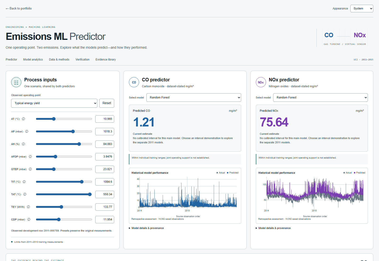
Luke Johnson · implemented application, captured during browser testing
From data to a working product
I undertook this personal project to gain practical experience with Python data analytics and machine learning, and to connect that learning with my engineering and software development background. Over approximately 2.5 working days, between 25 and 28 October 2026, I worked through an end-to-end example: data → analysis → models → verification and validation → product.
My overall goal was to deliver a functional application with data-driven models built in, while becoming more familiar with ML and data science approaches. I completed the workflow and deployed the application, using AI extensively for implementation and testing while directing the investigation, reviewing the evidence and shaping the product myself.
The task was to use historical measured plant data to build models that predict carbon monoxide (CO) and nitrogen oxides (NOx) emissions from nine concurrent gas-turbine measurements. The resulting web app lets visitors adjust operating inputs, compare model predictions and examine how those predictions performed against recorded emissions. These are estimates for a given operating condition, rather than forecasts of future emissions.
Read the results and discussion → for model descriptions, the complete later-year metric tables, verification findings and future work.
Understanding the data and choosing the method
I used the public UCI Gas Turbine CO and NOx Emission Data Set: 36,733 historical plant observations across 2011–2015, pairing measured operating conditions with recorded CO and NOx emissions. I reviewed distributions, correlations, operating patterns and unusual values before modelling. Humidity values above 100% and questions around published units were retained and flagged rather than silently corrected.
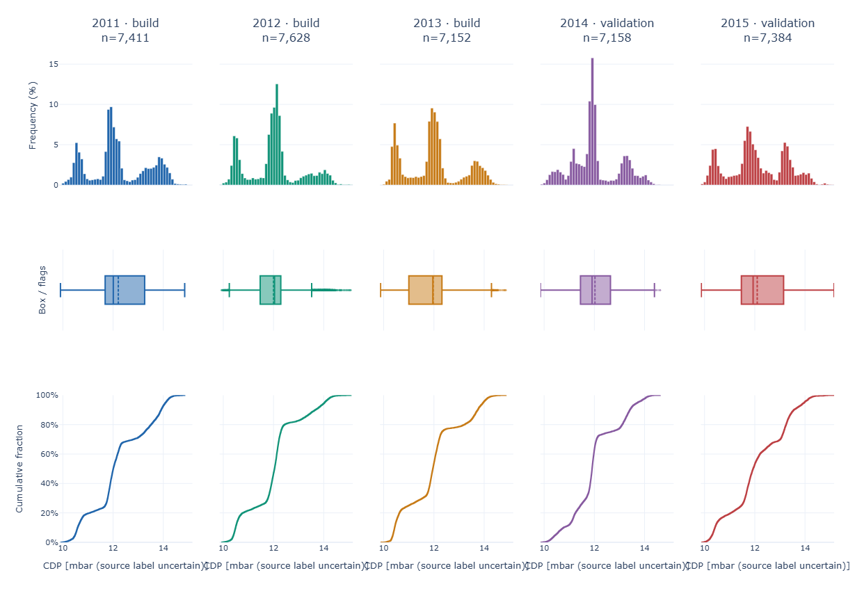
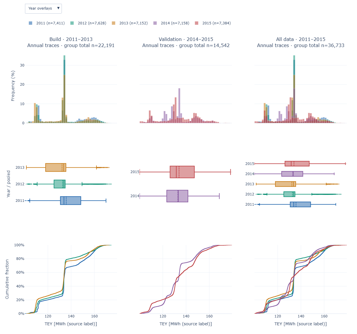
My initial review found broadly similar ranges and temporal behaviour across 2011–2013: recurring patterns and operating clusters, with no one development year looking wholly different. I flagged the AFDP rise in 2013, CDP tracking energy yield, and TAT concentrations near 550 and 525 for further investigation. This was a visual assessment, not proof that the annual distributions were identical.
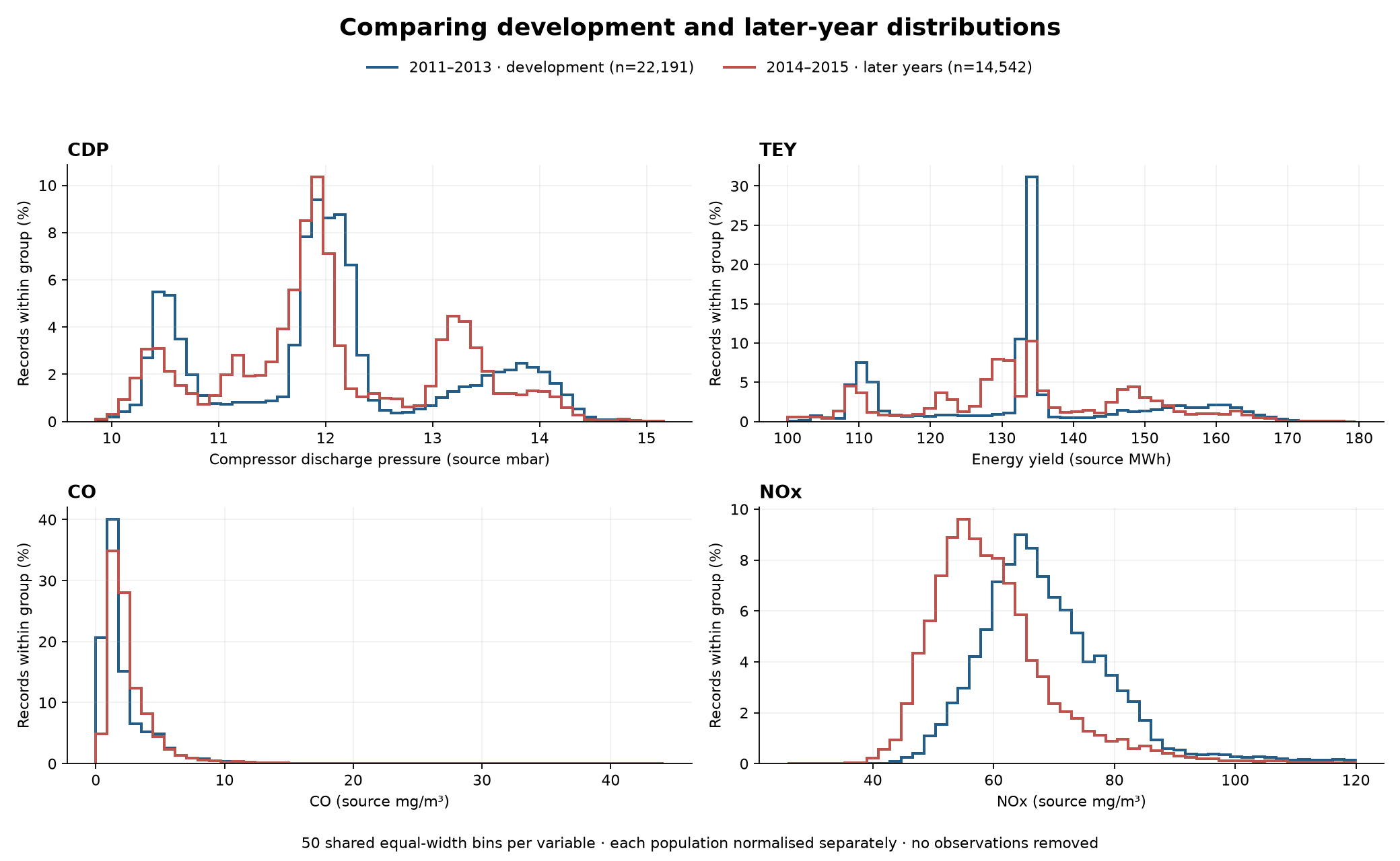
I also compared development (2011–2013) and later-year (2014–2015) populations. Broad overlap concealed important differences: later NOx mean concentration fell from 68.78 to 59.98 mg/m³, despite almost unchanged mean energy yield. Looking at distribution shapes as well as ranges helped challenge the initial impression of similarity.
I compared linear regression, histogram gradient boosting, a small neural network and Random Forest, with separate pipelines for each pollutant. Earlier years informed development; the main models fitted 2011–2013 and were assessed against 2014–2015. Keeping the chronology exposed changes that a random split could obscure.
Checking the calculations and challenging the results
I treated software verification and predictive validation as separate tasks. Checks covered metric arithmetic, data partitions, fitted transformations, saved-model replay and report behaviour. Verification caught a reversed residual-sign convention in a historical export; a corrected export preserved the original evidence.
Known-answer calculations used independent standard-library arithmetic, including deliberately awkward cases such as negative R², outliers and unequal group sizes. Replay and hash checks tested saved pipelines; interval checks reconstructed calibration ranks and coverage; browser checks tested report filters. The recorded final run contained 36,675 passed verification checks, alongside 162 pytest tests and eight browser-filter scenarios. These verify calculations and handling, rather than establishing predictive accuracy.
Results — what worked for CO and NOx
The strongest approach depended on the pollutant and assessment period. I compared four model families against the same chronological development folds, then reviewed the retained main models on 2014–2015. The original linear assessment was independently frozen; subsequent model comparisons used later years already inspected and are presented as retrospective.
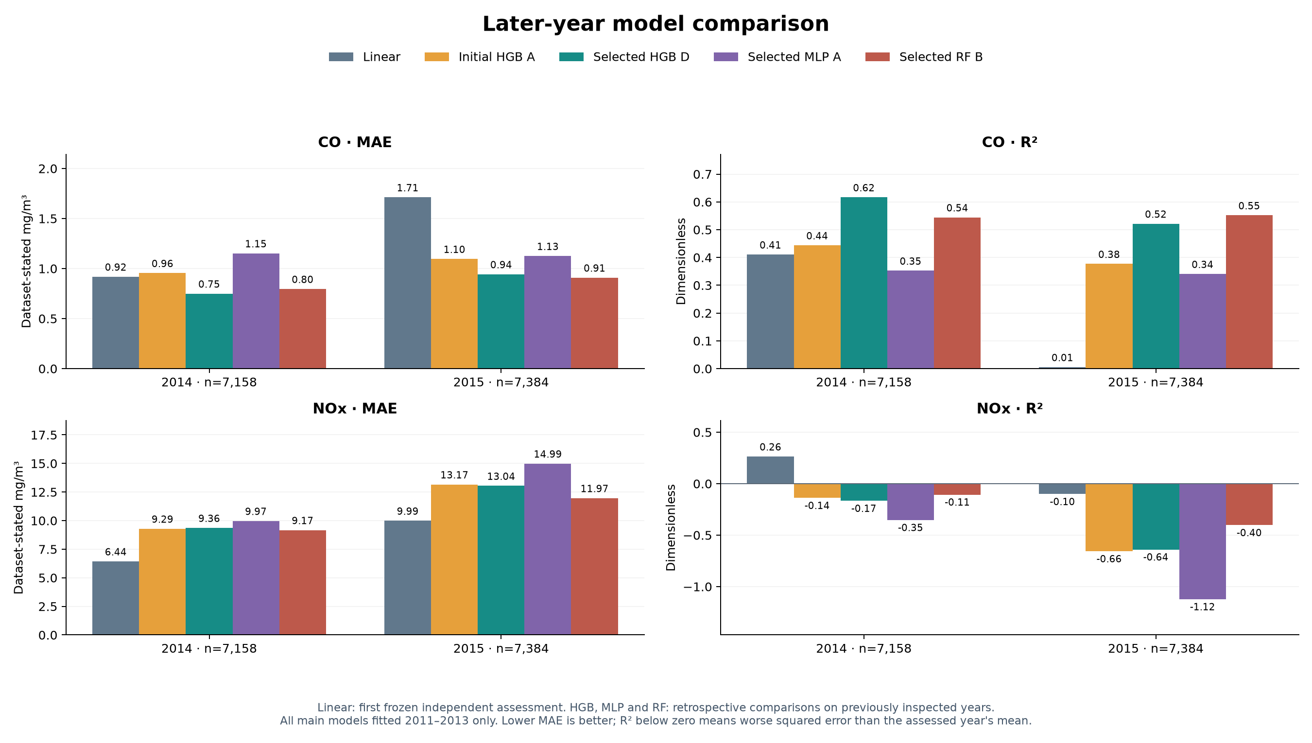
CO: tuned tree models gave the strongest later-year results. Selected histogram gradient boosting (HGB D) had the lowest development-fold MAE (0.830 mg/m³) and the best 2014 MAE (0.750) and R² (0.617). Selected Random Forest (RF B) was strongest in 2015 on MAE (0.910), RMSE (1.496) and R² (0.552), improving substantially on the linear baseline’s MAE of 1.713. This was useful predictive improvement, though neither model won every year and meaningful errors remained.
NOx: the simple linear baseline transferred best, despite stronger nonlinear development scores. The small multilayer perceptron (MLP A) had the lowest development-fold MAE (4.583 mg/m³), but linear regression had the lowest MAE and RMSE and highest R² in both later years. Its MAE was 6.437 in 2014 and 9.992 in 2015. Every nonlinear model had negative R² in both later years; even linear fell to −0.101 in 2015. The most successful approach for NOx in this comparison was therefore the linear baseline, with an important qualification: it still did not demonstrate reliable transfer across years.
| 2015 assessment | R² | MAE | RMSE |
|---|---|---|---|
| CO · Linear baseline | 0.005 | 1.713 | 2.229 |
| CO · Selected Random Forest B | 0.552 | 0.910 | 1.496 |
| NOx · Linear baseline | −0.101 | 9.992 | 11.682 |
| NOx · Selected Random Forest B | −0.403 | 11.969 | 13.185 |
MAE and RMSE use dataset-stated mg/m³; lower is better. R² is dimensionless, and negative values mean worse squared error than the assessed year’s mean. These selected 2015 rows illustrate the CO improvement and why the linear baseline remained preferable for later-year NOx. The full discussion includes all five main variants, both years, bias, tail errors and uncertainty assessments.
A separate prediction-interval exercise also tested whether the displayed uncertainty matched observed outcomes. Nominal 90% NOx intervals covered only 71.8–77.8% of the previously inspected 2013 evaluation records. That shortfall became part of the findings: producing an interval does not establish its reliability.
The NOx results suggest that the available inputs may not capture everything needed to transfer accurately between years. They do not prove which measurements or plant conditions are missing, or rule out model and measurement limitations. More complexity alone did not solve the problem.
For me, the useful finding was that model selection and validation need to follow the evidence separately for each output. CO showed a clear benefit from nonlinear models; NOx showed why a better development score alone is insufficient. The completed application lets a visitor explore both outcomes alongside the methods and retained assessments.
Making the investigation usable
I turned the retained models and analysis into a FastAPI application, with a TypeScript interface and interactive Plotly charts. Visitors adjust one shared operating scenario, select CO and NOx models independently, and explore estimates alongside historical performance, methods and verification evidence.
The app reuses the study’s fitted Python pipelines and functions. Separate interval demonstrations remain clearly identified, with input-range information and measured coverage visible. Responsive layouts and light/dark themes help make the technical material easier to explore. I deployed it in Docker on my Unraid server, behind the portfolio’s Nginx and Cloudflare Tunnel.
The browser sends named measurements and allowlisted model IDs to a FastAPI/Pydantic API. It never loads model files itself. The service validates requests and loads packaged pipelines, checking artifact hashes and the frontend/runtime manifest at startup. OpenAPI-generated TypeScript types connect the interface to the API contract, while Vite builds the frontend. Historical charts use saved predictions and stay separate from the visitor’s live scenario.
A preparation step packages public charts and evidence separately from private model artifacts. A multistage Docker build produces a non-root Python runtime, with catalogue, prediction, build-information and health endpoints. This kept the scientific implementation reusable while giving the demonstration a clear interface and traceable build.
Next steps
I would compare documented data corrections and several levels of outlier filtering against the unchanged baseline, with particular care not to hide genuine high-emission events. Further controlled model tuning and alternative algorithms are worthwhile, but need a fair chronological assessment. I would also conduct a structured literature review: I deliberately began with an open-ended familiarisation exercise, and now have my own evidence to compare with others’ approaches. The discussion page sets out the future work and initial reading references.
My contribution and what I learned
I used AI extensively for implementation, tests, documentation and iteration. I set the objectives, asked the engineering questions, reviewed plots and findings, and directed the product design and deployment. This was a practical exercise in learning new tools while retaining responsibility for the decisions and interpretation.
The outcome is a working, reviewable demonstration connecting analytical work to a usable product. It estimates concurrent emissions and remains an educational proof of concept; the study did not establish suitability for operational or regulatory monitoring. The most valuable learning was how to question a model’s outputs, retain evidence and communicate limitations alongside the result.
Project evidence
A closer look.
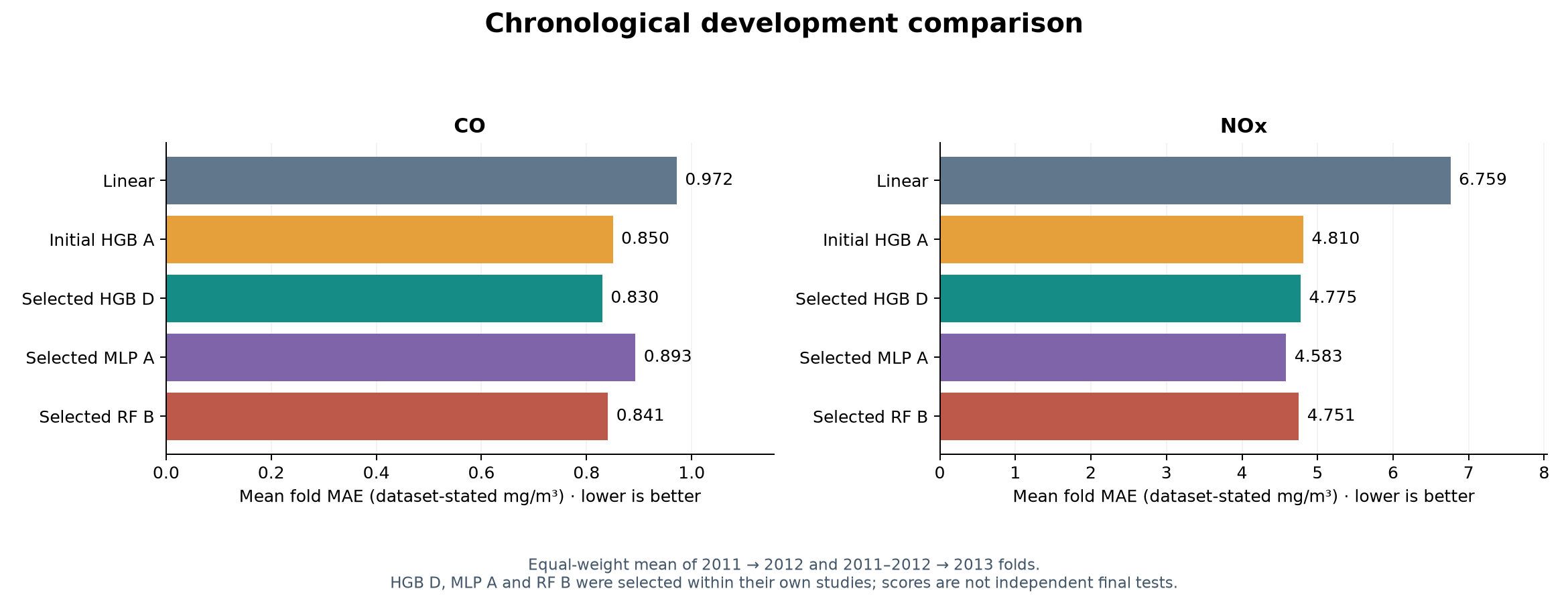
Development comparisons — mean absolute error over two chronological folds. These reused folds informed configuration selection; their scores are not unbiased final-test estimates.
Luke Johnson · generated from retained study metrics using MatplotlibLater-year performance — all main models fitted 2011–2013. The first frozen linear assessment was independent at the time; boosting, neural-network and Random Forest comparisons are retrospective on previously inspected years. Lower MAE is better; negative R² means worse squared error than the assessed year's mean.
Luke Johnson · generated from retained study metrics using MatplotlibFurther context
Technical references and related project information.