Personal project / Results & discussion
Gas Turbine Emissions — Results & Discussion.
A personal learning project connecting machine learning, engineering judgement and software development — from historical plant data to a working emissions-prediction application.
← Back to the project case study
From data to a working product
I undertook this personal project to gain practical experience with Python data analytics and machine learning, and to connect that learning with my engineering and software development background. Over approximately 2.5 working days, between 25 and 28 October 2026, I worked through an end-to-end example: data → analysis → models → verification and validation → product.
My overall aim was to produce a functional application with data-driven models built in: something a visitor could use to explore CO and NOx predictions, understand the inputs and review the supporting evidence. Becoming more familiar with ML and data science was central to the exercise. I used AI extensively to help implement and test the work, while I set the direction, reviewed the data and results, and shaped the interface.
I completed that workflow and deployed the application. The investigation records my approach to the problem, including the stronger CO results and the limitations exposed by NOx. The model findings are part of the learning, alongside delivering a usable product.
Study design and how to read the results
The task was to estimate concurrent CO and NOx concentrations from nine measured operating inputs. Development used 22,191 records from 2011–2013. Two forward-year folds fitted 2011 and assessed 2012, then fitted 2011–2012 and assessed 2013. Main models were subsequently fitted on all three development years. CO and NOx had separate pipelines; neither measured pollutant was an input to the other.
The first frozen linear assessment on 2014–2015 was independent at the time. Those years were subsequently inspected, so the later boosting, neural-network and forest comparisons are retrospective out-of-training assessments. They are useful evidence of transfer, but cannot become untouched tests again. No engineering acceptance tolerance was specified, so the study reports measured performance rather than an accuracy pass mark.
Input data review
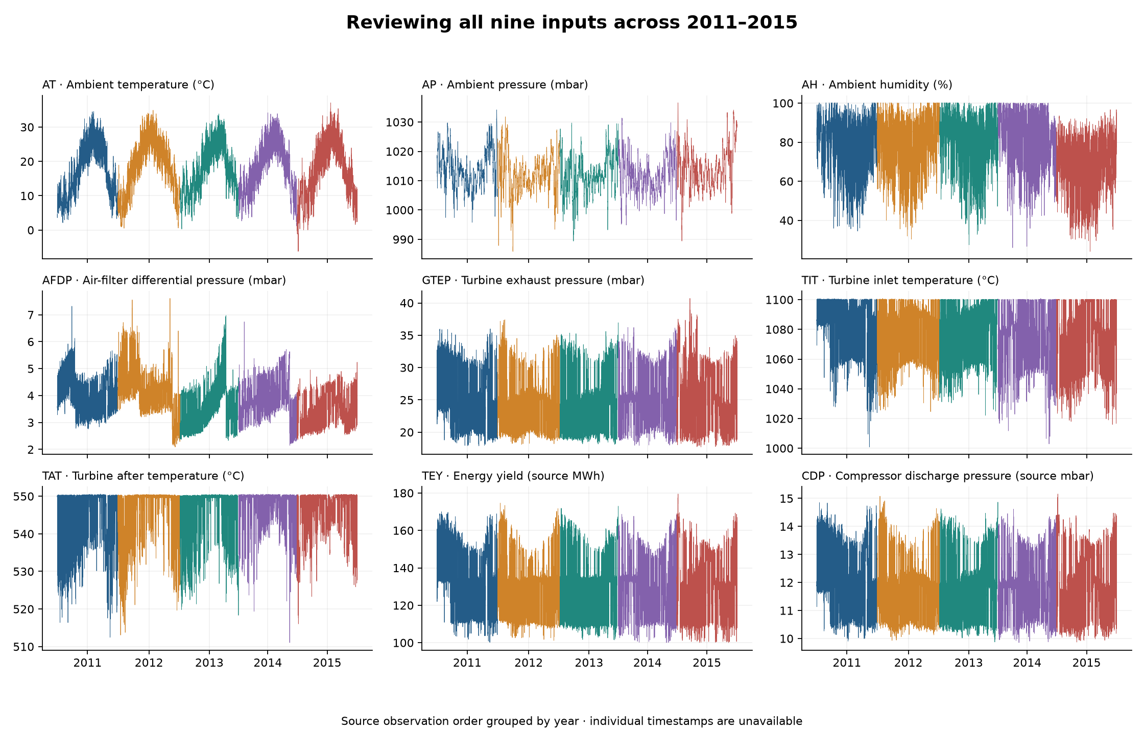
My initial visual review found broadly similar ranges and temporal behaviour across 2011–2013. There were patterns, cycles and operating clusters, but no single development year looked wholly exceptional. I noted an upward-curving AFDP section in 2013, energy-yield concentrations around 110 and 134–135, CDP broadly following energy yield, and TAT concentrated around 550 with lower readings near 525. These were observations to investigate, not established explanations or reasons to delete data.
Broad overlap did not mean identical populations. The grouped review compared 2011–2013 against 2014–2015, using common histogram bins and percentages within each group. Later NOx mean concentration was 59.98 versus 68.78 mg/m³, while mean energy yield was almost unchanged (133.46 versus 133.54, source-stated MWh). AFDP and other input distributions also differed. Similar ranges and similar means alone therefore gave incomplete reassurance.
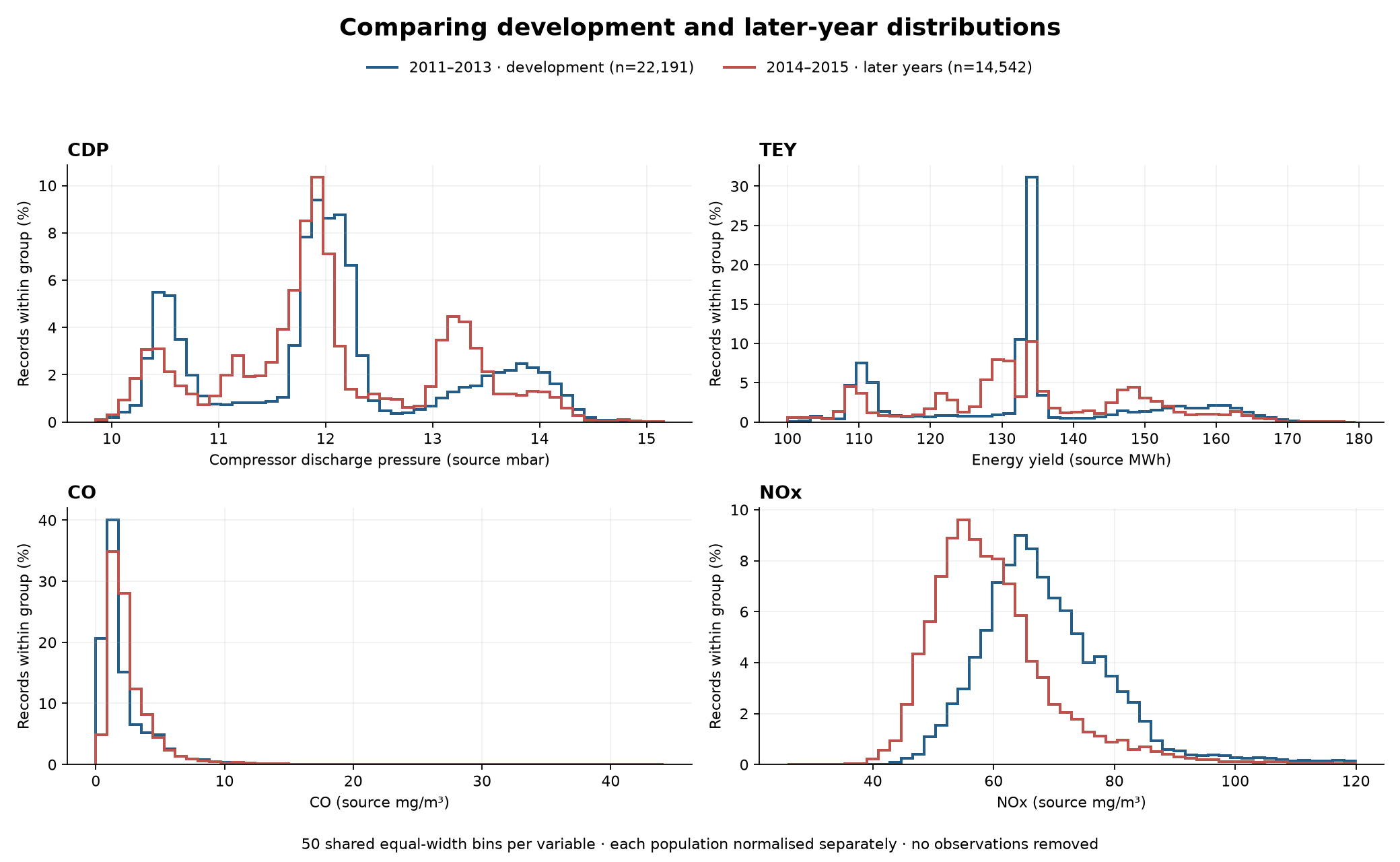
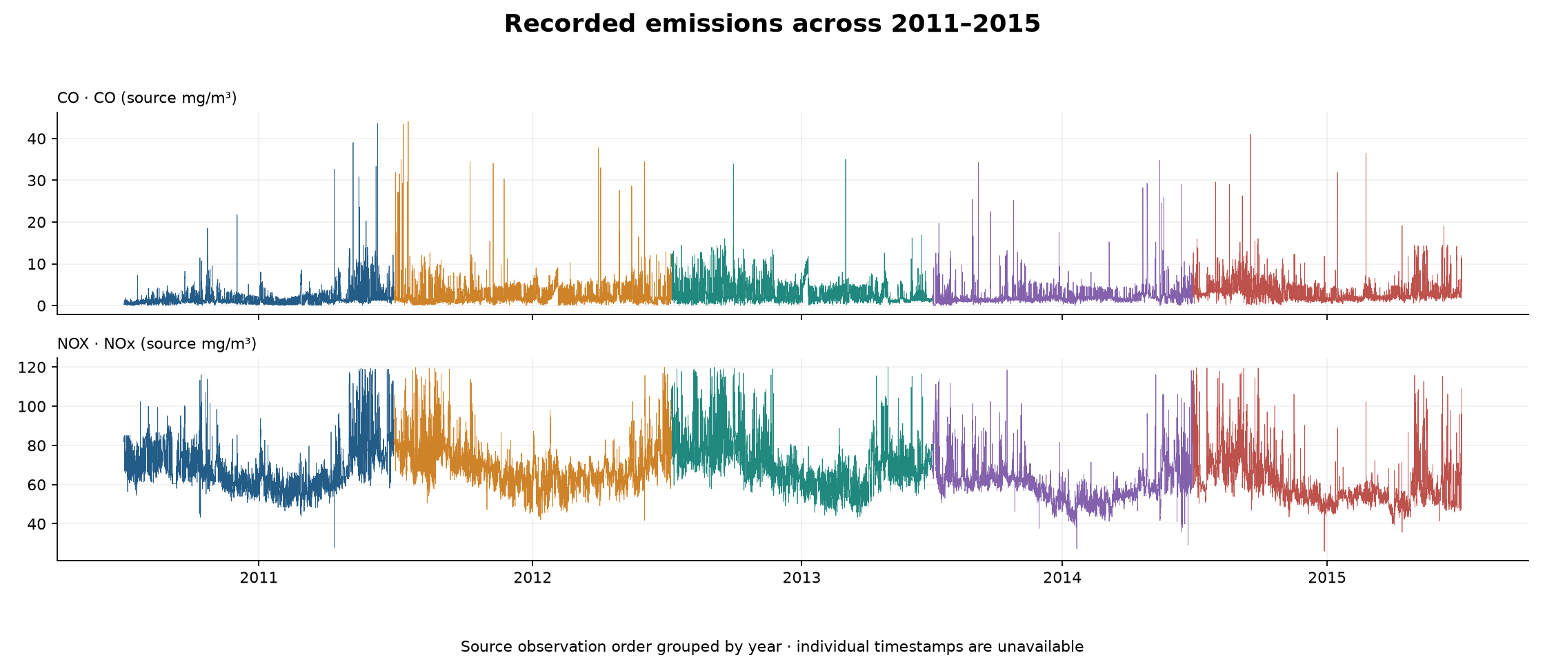
The review also checked completeness, duplicates, outlier flags and units. Humidity above 100% and questionable unit labels were recorded without invented corrections. High CO spikes were retained: a rare emission event is not automatically a bad measurement. An apparent NOx histogram discrepancy was investigated through 682 numerical comparisons, with no mismatches; annual peaks fell into different bins, explaining the lower pooled peak.
Models and methods
| Model and abbreviation | What it does | What I tried and learned |
|---|---|---|
| Linear regression | Fits a weighted linear relationship by least squares. | A transparent baseline with fitted input scaling. Later NOx was better than the nonlinear alternatives, though 2015 performance remained weak. |
| Histogram gradient boosting (HGB) | Builds successive decision trees to reduce prediction loss, grouping input values into bins. | Initial A plus four controlled configurations A–D. Development-fold MAE selected D for both pollutants. Improved CO transfer; did not resolve NOx. |
| Multilayer perceptron (MLP) | A neural network that learns nonlinear relationships through connected layers of weighted units. | Compared hidden layers (16), (32,16) and (64,32), with input and target scaling. Selected the small (16) network. Three seeds explored sensitivity; larger networks did not automatically improve results. |
| Random Forest (RF) | Averages many trees fitted to bootstrap samples. | Compared two 200-tree configurations. Selected B limited depth to 12, used at least 10 samples per leaf and considered 70% of features per split. Useful CO comparison; NOx still overpredicted. |
The results tables use Linear for linear regression, HGB for histogram gradient boosting, MLP for the multilayer perceptron and RF for Random Forest. Letters A–D identify configurations within a model study; “selected” means chosen using the development-fold rule below.
Configuration selection was independent for each pollutant: lowest unweighted mean of the two fold MAEs, with RMSE then configuration label breaking ties. Main fits used the selected settings and retained their preprocessing. The comparison reused the same chronological folds; its winning scores are development evidence, not unbiased final-test estimates.
| Main variant | CO mean fold MAE | NOx mean fold MAE |
|---|---|---|
| Linear | 0.972 | 6.759 |
| Initial HGB A | 0.850 | 4.810 |
| Selected HGB D | 0.830 | 4.775 |
| Selected MLP A | 0.893 | 4.583 |
| Selected RF B | 0.841 | 4.751 |
Errors use dataset-stated mg/m³. Boosting D had the lowest CO development MAE; MLP A had the lowest NOx development MAE. Neither ranking established an overall best model for later years.
Later-year performance
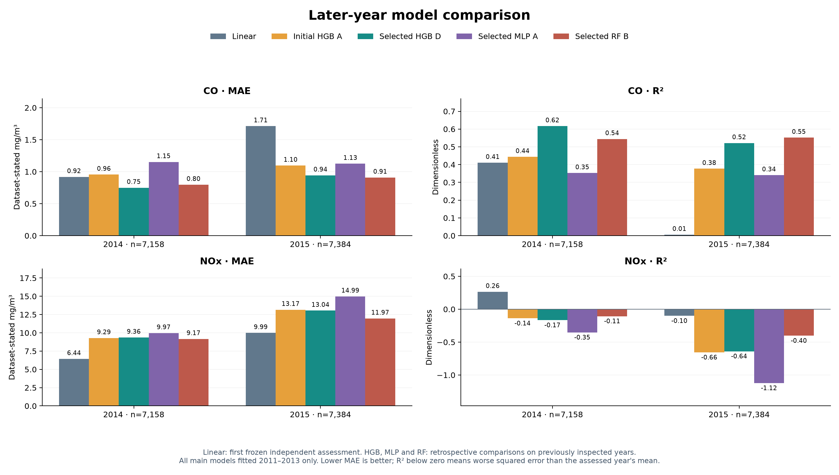
The tables below reproduce the saved metric overview, rounded to three decimals. 2014: n=7,158; 2015: n=7,384 for every model. All main models fitted 2011–2013 only. Linear rows are the original independent assessment; all other rows are retrospective comparisons on previously inspected years.
CO — later-year results
| Model | Year | R² | MAE | RMSE | Bias | P95 error | Negative predictions |
|---|---|---|---|---|---|---|---|
| Linear | 2014 | 0.411 | 0.919 | 1.541 | -0.520 | 2.332 | 1462 |
| Linear | 2015 | 0.005 | 1.713 | 2.229 | -1.626 | 3.590 | 2229 |
| Initial HGB A | 2014 | 0.444 | 0.955 | 1.497 | 0.623 | 2.545 | 0 |
| Initial HGB A | 2015 | 0.377 | 1.096 | 1.764 | -0.434 | 2.720 | 0 |
| Selected HGB D | 2014 | 0.617 | 0.750 | 1.242 | 0.401 | 2.088 | 0 |
| Selected HGB D | 2015 | 0.522 | 0.944 | 1.546 | -0.647 | 2.240 | 0 |
| Selected MLP A | 2014 | 0.352 | 1.153 | 1.615 | 0.777 | 2.951 | 10 |
| Selected MLP A | 2015 | 0.341 | 1.126 | 1.815 | -0.318 | 3.130 | 74 |
| Selected RF B | 2014 | 0.544 | 0.796 | 1.355 | 0.470 | 2.295 | 0 |
| Selected RF B | 2015 | 0.552 | 0.910 | 1.496 | -0.520 | 2.118 | 0 |
NOx — later-year results
| Model | Year | R² | MAE | RMSE | Bias | P95 error | Negative predictions |
|---|---|---|---|---|---|---|---|
| Linear | 2014 | 0.265 | 6.437 | 8.550 | 3.228 | 17.516 | 0 |
| Linear | 2015 | -0.101 | 9.992 | 11.682 | 8.362 | 20.837 | 0 |
| Initial HGB A | 2014 | -0.139 | 9.291 | 10.642 | 8.251 | 17.980 | 0 |
| Initial HGB A | 2015 | -0.657 | 13.165 | 14.328 | 13.042 | 21.759 | 0 |
| Selected HGB D | 2014 | -0.167 | 9.361 | 10.772 | 8.296 | 18.060 | 0 |
| Selected HGB D | 2015 | -0.640 | 13.040 | 14.253 | 12.906 | 22.136 | 0 |
| Selected MLP A | 2014 | -0.353 | 9.973 | 11.600 | 9.251 | 19.607 | 0 |
| Selected MLP A | 2015 | -1.123 | 14.987 | 16.219 | 14.905 | 25.757 | 0 |
| Selected RF B | 2014 | -0.106 | 9.169 | 10.487 | 8.051 | 17.703 | 0 |
| Selected RF B | 2015 | -0.403 | 11.969 | 13.185 | 11.730 | 20.263 | 0 |
Reading the measures: MAE is average absolute error; RMSE weights larger errors more strongly; P95 error is the 95th percentile of absolute error. Bias here is predicted minus measured, so positive values indicate overprediction. Those four quantities use dataset-stated mg/m³. R² is dimensionless: 1 is perfect, 0 matches the assessed population’s mean in squared-error terms, and negative values are worse. It is not percentage accuracy. Negative-prediction counts expose physically implausible outputs; predictions were not silently clipped. The app’s residual charts use the separately labelled measured minus predicted convention.
Download the full saved overview CSV, including training diagnostics, exact values, sample counts and source-file paths.
What worked, and what did not
For CO, selected HGB D reduced 2014 MAE from the linear baseline’s 0.919 to 0.750 mg/m³. Selected RF B had the lowest 2015 CO MAE among these variants (0.910), with R² 0.552. This was useful improvement, with substantial residual errors still visible. No single variant won every metric and year.
For NOx, nonlinear training R² reached approximately 0.82–0.89, yet every nonlinear variant had negative later-year R². In 2015, MLP A had MAE 14.987 and bias +14.905 mg/m³: systematic overprediction was a major part of its error. The simpler linear baseline was better on later-year NOx MAE, but its 2015 R² was still −0.101. Better training fit and competitive development scores had not delivered reliable transfer.
Other assessments and uncertainty
| Assessment | What it checked | Recorded outcome and interpretation |
|---|---|---|
| Training fit (Check A) | Predictions on fitting records, separate from later-year evaluation. | Nonlinear fits improved markedly; this did not establish generalisation. |
| Prediction repeatability (Check B) | Repeated calls, reloads, a fresh Python process and saved predictions. | All ten original linear comparisons had zero observed maximum difference. Repeatable predictions can still be inaccurate. |
| Simple reference | Predict the earlier training population’s mean. | Linear beat the reference on three of four target/year MAEs; CO 2015 was worse (1.713 versus 1.386). |
| Tail and operating-condition errors | Training-derived emission P90 thresholds and TEY/TIT/AT bins. | Evaluated difficult regions rather than only global averages. RF B’s improved mean development MAE did not improve every high-emission diagnostic. |
| Input envelope | Compare later measurements with training min/max ranges. | Only 7 rows in 2014 and 111 in 2015 exceeded any range, despite substantial errors. Individual bounds did not establish joint support or accuracy. |
| MLP seed sensitivity | Repeat selected architecture with seeds 17, 42 and 73. | Some fitting variation; the broader NOx difficulty remained. Seed 42 was retained rather than selecting a favourable seed. |
| Interval reproduction | Reload separate fitted/calibrated artifacts and replay 2013 predictions and bounds. | Exact reproduction for all 16 family/target/coverage combinations; this checked implementation, not achieved coverage. |
The separate split-conformal experiment fitted 2011, calibrated absolute residuals on 2012 and evaluated 7,152 previously inspected 2013 records. It did not attach uncertainty margins to the main 2011–2013 models. Each family/target/level has a constant-width interval, with bounds retained even when negative. Temporal dependence and distribution changes can undermine the assumptions behind nominal coverage.
| Interval model | CO coverage at nominal 90% / 95% | NOx coverage at nominal 90% / 95% |
|---|---|---|
| Linear | 79.1% / 88.5% | 71.8% / 80.9% |
| Original fixed HGB | 85.8% / 92.0% | 77.8% / 85.6% |
| Random Forest A | 90.9% / 95.8% | 75.1% / 85.4% |
| MLP A, seed 42 | 82.7% / 89.5% | 74.5% / 83.2% |
Every NOx model undercovered at both levels. Forest CO exceeded both nominal levels with the widest CO intervals, illustrating a coverage-versus-width trade-off. A nominal 90% interval is not a claim that a particular prediction is “90% certain”.
Method verification — checking the implementation
I checked the calculations and data handling against known answers, rather than assuming that using an established library made the complete workflow correct. Independent arithmetic references used Python’s standard library to test MAE, RMSE, R² and bias, including negative R², balanced errors, outliers and unequal group sizes. Checks distinguished pooled metrics from equal-fold averages and confirmed sign conventions. Data tests checked row identity, chronological membership, target exclusion and fitted transformations; artifact checks replayed saved pipelines and compared hashes before and after prediction. For the interval method, checks reconstructed calibration scores, exact conformal ranks, bounds and coverage counts. Browser scenarios checked that report filters displayed the intended populations.
The 28 October 2026 recorded execution reported 36,675 passed verification checks, zero failed or incomplete, a 162-test pytest suite, and eight passing browser-filter scenarios. These are different categories of evidence, not interchangeable or additive test counts. Verification found two historical MLP residual columns using the opposite sign: the original export was preserved and a corrected export provided. Predictions and aggregate performance were unaffected. These checks support the implementation and reporting; they do not verify sensor calibration, prove the chosen model is adequate, or establish operational suitability.
Conclusion — a completed workflow and contrasting prediction results
I achieved the overall project goal: a working web application with retained data-driven models, connected to the analysis, checks and evidence behind them. It gave me practical experience of taking an unfamiliar ML problem through to a usable product, while applying the engineering habit of questioning what a result actually demonstrates.
CO prediction was the stronger result. Selected boosting reduced 2014 MAE from 0.919 to 0.750 mg/m³, while selected Random Forest reduced 2015 MAE from 1.713 to 0.910 mg/m³ and raised R² from 0.005 to 0.552. The nonlinear models captured useful relationships and improved on the linear baseline, although meaningful errors remained and no model won every metric and year. These later nonlinear comparisons remain retrospective.
The models tested did not demonstrate reliable NOx prediction across years. The results are consistent with changing relationships between the available measurements and emissions. The nine inputs may not capture all the information needed for accurate transfer, but that remains a hypothesis: this exercise cannot distinguish missing explanatory variables from measurement changes, operating changes, model limitations or other causes. Broadly similar ranges did not ensure that the learned relationship remained valid.
For me, that contrast is a useful outcome of the exercise: I learned how to build and verify the workflow, recognise where a model helps, and communicate where it falls short. The application makes both outcomes inspectable. Further work can build on this completed demonstration without presenting either pollutant model as ready for operational monitoring.
Future work
- Data quality and outlier sensitivity. Resolve documented units and suspicious measurements where source evidence permits. Compare the unchanged baseline with several predeclared levels of outlier filtering or robust fitting. Define thresholds on fitting data only, record every exclusion and retain an unfiltered assessment, including high-emission events. Removing difficult records must not become a way to manufacture better scores.
- Further tuning and alternative methods. Extend controlled searches for tree depth, leaf size, learning rate and regularisation, and revisit MLP scaling and architecture. Candidates could include Extra Trees, support-vector regression, nearest neighbours and alternative boosting implementations. Compare them under the same chronological protocol, with explicit point-error and interval-coverage objectives. New choices informed by these results need genuinely new assessment data before being described as independently validated.
- Investigate what is missing. Examine residuals against operating regimes and joint input support, and seek plant context or additional measurements if available. Test possible explanations rather than attributing the NOx shift to an assumed plant event.
- Conduct a structured literature review. I deliberately approached the modelling as an open-ended familiarisation exercise rather than beginning with published solutions. With my own evidence now available, reviewing others’ findings could suggest different ways to analyse the dataset. A preliminary reference list exists; this is still future comparative work, not a completed systematic review or evidence that my scores match published benchmarks.
Starting points for that review
| Reference | Reason to review |
|---|---|
| Kaya, Tüfekci & Uzun (2019), Predicting CO and NOx emissions from gas turbines: novel data and a benchmark PEMS | Original dataset paper and benchmark procedure. |
| Kochueva & Nikolskii (2021), Data Analysis and Symbolic Regression Models for Predicting CO and NOx Emissions from Gas Turbines | Data review and explicit equation-based alternatives. |
| Wood (2023), Long-term atmospheric pollutant emissions from a combined cycle gas turbine: Trend monitoring and prediction applying machine learning | Multiyear changes and comparisons across regression methods. |
| Rodríguez-Abreo et al. (2026), Reliability-Oriented Predictive Emission Monitoring of Gas Turbines Under Multiyear Distribution Shift and High-Emission Tail Risk | Chronological evaluation, calibration and high-emission performance. |
For each paper I would record inputs, cleaning, training/selection/test years, calibration and metric definitions before comparing results. Random within-period splits, forward-year tests and later-year calibration answer different questions. These reading references are leads supplied after the exercise, not external validation of my conclusions.
Evidence sources
Values and figures are drawn from the retained study’s model-results overview, chronological measurement export, grouped histogram bins, uncertainty evaluation and recorded verification summary. Figures were rendered from saved evidence without retraining or new predictions. Dataset: UCI Gas Turbine CO and NOx Emission Data Set, CC BY 4.0. The application’s evidence library provides access to the underlying methods and reports.